| Line 14: | Line 14: | ||
# Execute a run of the simulator. At the command prompt enter [t,x,d,te,z,e] = NetworkSimRun(tF,Dat); | # Execute a run of the simulator. At the command prompt enter [t,x,d,te,z,e] = NetworkSimRun(tF,Dat); | ||
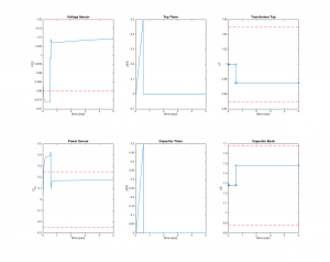
# Note that every time you call the function a series of plots is also generated. You may want to comment this out later. For now, check to maker sure your plots agree with the reference plot below. | # Note that every time you call the function a series of plots is also generated. You may want to comment this out later. For now, check to maker sure your plots agree with the reference plot below. | ||
| − | [[File:NetworkSimRun_SamplePlot.png| | + | [[File:NetworkSimRun_SamplePlot.png|300px|right|Simulation sample plot.]] |
Revision as of 10:55, 23 November 2017
In this exercise you will connect your FSA files with the continuous dynamics.
Step 1: Download the simulator files using the link below and unzip them into a common folder.
- Step 2: Supplement the simulator files with your FSA files. The simulator is missing the following FSA files that you will have to provide (note, these files have no extensions, which means your files should not have an extension either, i.e., no .txt or similar):
- T_6sup - the tap changer supervisor automata
- T_switch - the tap changer automata
- T_sensor - the voltage sensor automata
- T_timer - the tap changer timer automata
- Step 3: Test to make sure that the hybrid simulator works correctly.
- Define the parameter perturbation vector: Dat = [0.0488; 2.4399; 3.3427];
- Execute a run of the simulator. At the command prompt enter [t,x,d,te,z,e] = NetworkSimRun(tF,Dat);
- Note that every time you call the function a series of plots is also generated. You may want to comment this out later. For now, check to maker sure your plots agree with the reference plot below.
